
Microsoft Power BI is an interactive data analysis and visualization tool that’s used for business intelligence (BI) and that you can now script with Python. By combining these two technologies, you can extend Power BI’s data ingestion, transformation, augmentation, and visualization capabilities. In addition, you’ll be able to bring complex algorithms shipped with Python’s numerous data science and machine learning libraries to Power BI.
In this tutorial, you’ll learn how to:
- Install and configure the Python and Power BI environment
- Use Python to import and transform data
- Make custom visualizations using Python
- Reuse your existing Python source code
- Understand the limitations of using Python in Power BI
Whether you’re new to Power BI, Python, or both, you’ll learn how to use them together. However, it would help if you knew some Python basics and SQL to benefit fully from this tutorial. Additionally, familiarity with the pandas and Matplotlib libraries would be a plus. But don’t worry if you don’t know them, as you’ll learn everything you need on the job.
While Power BI has potential across the world of business, in this tutorial, you’ll focus on sales data. Click the link below to download a sample dataset and the Python scripts that you’ll be using in this tutorial:
Source Code: Click here to get the free source code and dataset that you’ll use to combine Python and Power BI for superpowered business insights.
Preparing Your Environment
To follow this tutorial, you’ll need Windows 8.1 or later. If you’re currently using macOS or a Linux distribution, then you can get a free virtual machine with an evaluation release of the Windows 11 development environment, which you can run through the open-source VirtualBox or a commercial alternative.
Note: The Windows image weighs approximately 20 gigabytes, so it can take a long time to download and install. Beware of the fact that running another operating system in a virtual machine will require a considerable amount of computer memory.
In this section, you’ll install and configure all the necessary tools to run Python and Power BI. By the end of it, you’ll be ready to integrate Python code into your Power BI reports!
Install Microsoft Power BI Desktop
Microsoft Power BI is a collection of various tools and services, some of which require a Microsoft account, a subscription plan, and an Internet connection. Fortunately for you, in this tutorial, you’ll use Microsoft Power BI Desktop, which is completely free of charge, doesn’t require a Microsoft account, and can work offline just like a traditional office suite.
There are a few ways in which you can obtain and install Microsoft Power BI Desktop on your computer. The recommended approach, which is arguably the most convenient one, is to use Microsoft Store, accessible from the Start menu or its web-based storefront:
By installing Power BI Desktop from the Microsoft Store, you’ll ensure automatic and quick updates to the latest Power BI versions without having to be logged in as the system’s administrator. However, if that method doesn’t work for you, then you can always try downloading the installer from the Microsoft Download Center and running it manually. The executable file is roughly four hundred megabytes in size.
Once you have the Power BI Desktop application installed, launch it, and you’ll be greeted with a welcome screen similar to the following one:
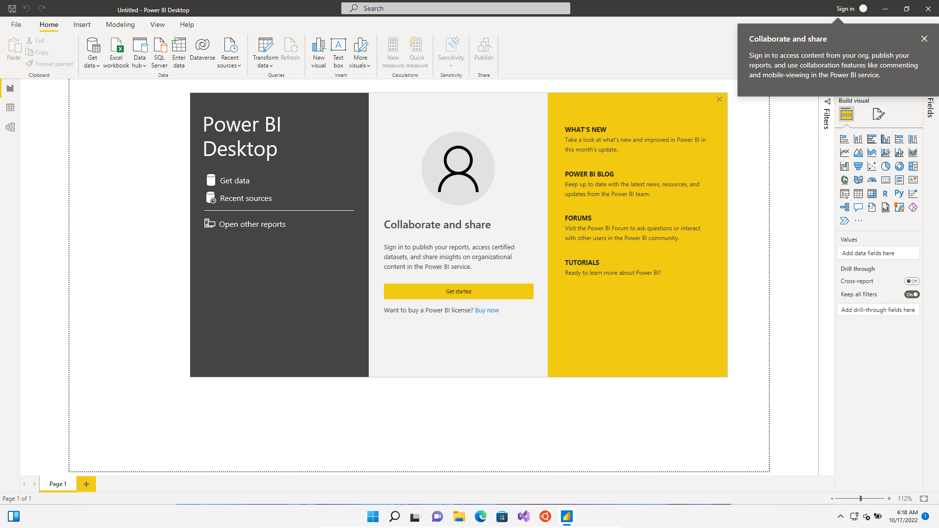
Don’t worry if the Power BI Desktop user interface feels intimidating at first. You’ll get to know the basics as you make your way through the tutorial.
Install Microsoft Visual Studio Code
Microsoft Power BI Desktop offers only rudimentary code editing features, which is understandable since it’s mainly a data analysis tool. It doesn’t have intelligent contextual suggestions, auto-completion, or syntax highlighting for Python, all of which are invaluable when working with code. Therefore, you should really use an external code editor for writing anything but the most straightforward Python scripts in Power BI.
Feel free to skip this step if you already use an IDE like PyCharm or if you don’t need any of the fancy code editing features in your workflow. Otherwise, consider installing Visual Studio Code, which is a free, modern, and extremely popular code editor. Because it’s made by Microsoft, you can quickly find it in the Microsoft Store:
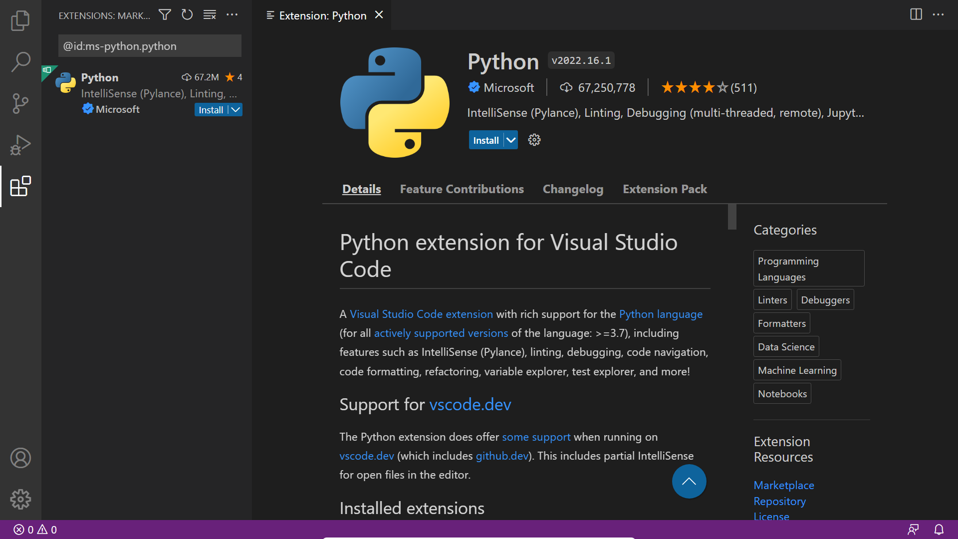
Microsoft Visual Studio Code, or VS Code as some like to call it, is a universal code editor that supports many programming languages through extensions. It doesn’t understand Python out of the box. But when you open an existing file with Python source code or create a new file and select Python as the language in VS Code, then it’ll prompt you to install the recommended set of extensions for Python:
After you confirm and proceed, VS Code will ask you to specify the path to your Python interpreter. In most cases, it’ll be able to detect one for you automatically. If you haven’t installed Python on your computer yet, then check out the next section, where you’ll also get your hands on pandas and Matplotlib.
Install Python, pandas, and Matplotlib
Now it’s time to install Python, along with a couple of libraries required by Power BI Desktop to make your Python scripts work in this data analysis tool.
If you’re a data analyst, then you may already be using Anaconda, a popular Python distribution that bundles hundreds of scientific libraries and a custom package manager. Data analysts tend to choose Anaconda over the standard Python distribution because it makes their environment setup more convenient. Ironically, setting up Anaconda with Power BI Desktop is more cumbersome than using standard Python, and it’s not even recommended by Microsoft:
Distributions that require an extra step to prepare the environment (for example, Conda) might encounter an issue where their execution fails. We recommend using the official Python distribution from https://www.python.org/ to avoid related issues. (Source)
Anaconda usually uses the release of Python a few generations back, which is another reason to prefer the standard distribution if you want to stay on the cutting edge. That said, you’ll find some help on how to use Anaconda and Power BI Desktop in the next section.
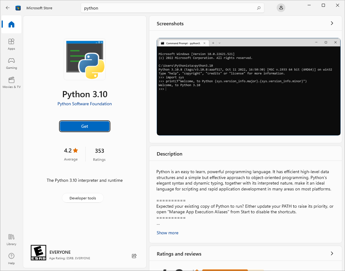
If you’re starting from scratch without having installed Python on your computer before, then your best option is to use Microsoft Store again. Find the most recent Python release and proceed with installing it:
When the installation is complete, you’ll see a couple of new entries in your Start menu. It’ll also make the python command immediately available to you in the command prompt, along with pip for installing third-party Python packages.
Note: You’ll be using Windows Terminal in this tutorial, which comes installed by default on Windows 11. If you’re on Windows 10 or below, then take a minute to install Windows Terminal manually from Microsoft Store. In a nutshell, Windows Terminal is a universal container that can host multiple shells, such as PowerShell.
Power BI Desktop requires your Python installation to have two extra libraries, pandas and Matplotlib, which aren’t provided as standard unless you’ve used Anaconda. However, installing third-party packages into the global or system-wide Python interpreter is considered a bad practice. Besides, you wouldn’t be able to run the system interpreter from Power BI due to permission restrictions on Windows. You need a Python virtual environment instead.
A virtual environment is a folder that contains a copy of the global Python interpreter, which you’re free to mess around with. You can install extra libraries into it without worrying about breaking other programs that might also depend on Python. At any point, you can safely remove the folder containing your virtual environment and still have Python on your computer afterward.
PowerShell forbids running scripts by default, including those for managing Python virtual environments, because of a restricted execution policy that’s in place. Before you can activate your virtual environment, there’s some initial setup required. Go to your Start menu, find Windows Terminal, right-click on it, choose Run as administrator, and confirm by clicking Yes. Next, type the following command to elevate your execution policy:
PS> Set-ExecutionPolicy RemoteSigned
Make sure you’re running this command as the system administrator in case of any errors.
The RemoteSigned policy will allow you to run local scripts as well as scripts downloaded from the Internet as long as they’re signed by a trusted authority. This configuration needs to be done only once, so you can close the window now. However, there’s much more to setting up a Python coding environment on Windows, so feel free to check out the guide if you’re interested.
Now, it’s time to pick a parent folder for your virtual environment. It could be in your workspace for Power BI reports, for example. However, if you’re unsure where to put it, then you can use your Windows user’s Desktop folder, which is quick to locate. In such a case, right-click anywhere on the desktop and choose the Open in Terminal option. This will open the Windows Terminal with your desktop as the current working directory.
Next, use Python’s venv module to create a new virtual environment in a local folder. You can name the folder powerbi-python to remind yourself of its purpose later:
PS> python -m venv powerbi-python
After a few seconds, there will be a new folder with a copy of the Python interpreter on your desktop. Now, you can activate the virtual environment by running its activation script and then install the two libraries expected by Power BI. Type the following two commands while the desktop is still your current working directory:
PS> .\powerbi-python\Scripts\activate
(powerbi-python) PS> python -m pip install pandas matplotlib
After activating it, you should see your virtual environment’s name, powerbi-python, in the prompt. Otherwise, you’d be installing third-party packages into the global Python interpreter, which is what you wanted to avoid in the first place.
All right, you’re almost set. You can repeat the two steps of activating your virtual environment and using pip to install other third-party packages if you feel like adding more libraries to your environment. Next up, you’ll tell Power BI where to find Python in your virtual environment.
Configure Power BI Desktop for Python
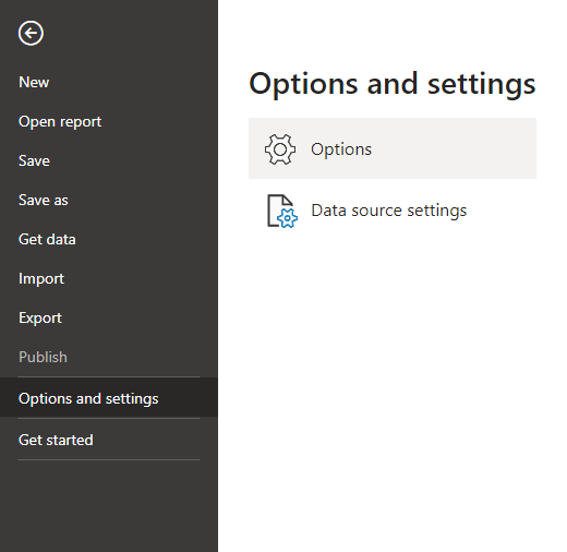
Return to Power BI Desktop or, if you’ve already closed it, start it again. Dismiss the welcome screen by clicking the X icon in the top-right corner of the window, and select Options and Settings from the File menu. Then, go to Options, which has a gear icon next to it:
This will reveal a number of configuration options grouped by categories. Click the group labeled Python scripting in the column on the left, and set the Python home directory by clicking the Browse button depicted below:
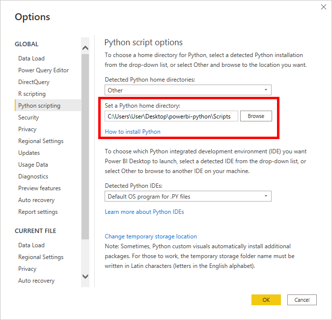
You must specify the path to the Scripts subfolder, which contains the python.exe executable, in your virtual environment. If you put the virtual environment in your Desktop folder, then your path should look something like this:
C:\Users\User\Desktop\powerbi-python\Scripts
Replace User with whatever your username is. If the specified path is invalid and doesn’t contain a virtual environment, then you’ll get a suitable error message.
If you have Anaconda or its stripped-down Miniconda flavor on your computer, then Power BI Desktop should detect it automatically. Unfortunately, in order for it to work correctly, you’ll need to start the Anaconda Prompt from the Start menu and manually create a separate environment with the two required libraries first:
(base) C:\Users\User> conda create --name powerbi-python pandas matplotlib
This is similar to setting up a virtual environment with the regular Python distribution and using pip to install third-party packages.
Next, you’ll want to list your conda environments and take note of the path to your newly created powerbi-python one:
(base) C:\Users\User> conda env list
# conda environments:
#
base                  *  C:\Users\User\anaconda3
powerbi-python           C:\Users\User\anaconda3\envs\powerbi-python
Copy the corresponding path and paste it into Power BI’s configuration to set the Python home folder option. Note that with a conda environment, you don’t need to specify any subfolder, because the Python executable is located right inside the environment’s parent folder.
While still in the Python scripting options, you’ll find another interesting configuration down below. It lets you specify the default Python IDE or code editor that Power BI should launch for you when you’re writing a code snippet. You can keep the operating system’s default program associated with the .py file extension or you can indicate a specific Python IDE of your choice:
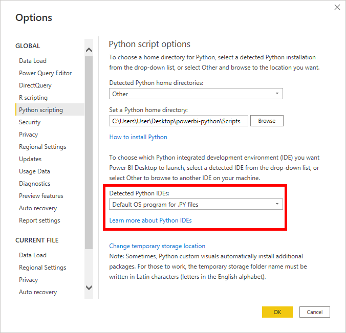
To specify your favorite Python IDE, select Other from the first dropdown and browse to the executable file of your code editor, such as this one:
C:\Users\User\AppData\Local\Programs\Microsoft VS Code\Code.exe
As before, the correct path on your computer might be different. For more details on using an external Python IDE with Power BI, check out the online documentation.
Congratulations! That concludes the configuration of Power BI Desktop for Python. The most important setting is the path to your Python virtual environment, which should contain the pandas and Matplotlib libraries. In the next section, you’ll see Power BI and Python in action.
Running Python in Power BI
There are three ways to run Python code in Power BI Desktop, which integrate with the typical workflow of a data analyst. Specifically, you can use Python as a data source to load or generate datasets in your report. You can also perform cleaning and other transformations of any dataset in Power BI using Python. Finally, you can leverage Python’s plotting libraries to create data visualizations. You’ll get a taste of all these applications now!
Data Source: Import a pandas.DataFrame
Suppose you must ingest data from a proprietary or a legacy system that Power BI doesn’t support. Maybe your data is stored in an obsolete or not-so-popular file format. In any case, you can whip up a Python script that’ll glue the two parties together through one or more pandas.DataFrame objects.
A DataFrame is a tabular data storage format, much like a spreadsheet or a table in a relational database. It’s two-dimensional and consists of rows and columns, where each column typically has an associated data type, such as a number or date. Power BI can grab data from Python variables holding pandas DataFrames, and it can inject variables with DataFrames back into your script.
In this tutorial, you’ll use Python to load fake sales data from SQLite, which is a widespread file-based database engine. Note that it’s technically possible to get such data directly in Power BI Desktop, but only after installing a suitable SQLite driver and using the ODBC connector. On the other hand, Python supports SQLite right out of the box, so choosing it may be more convenient.
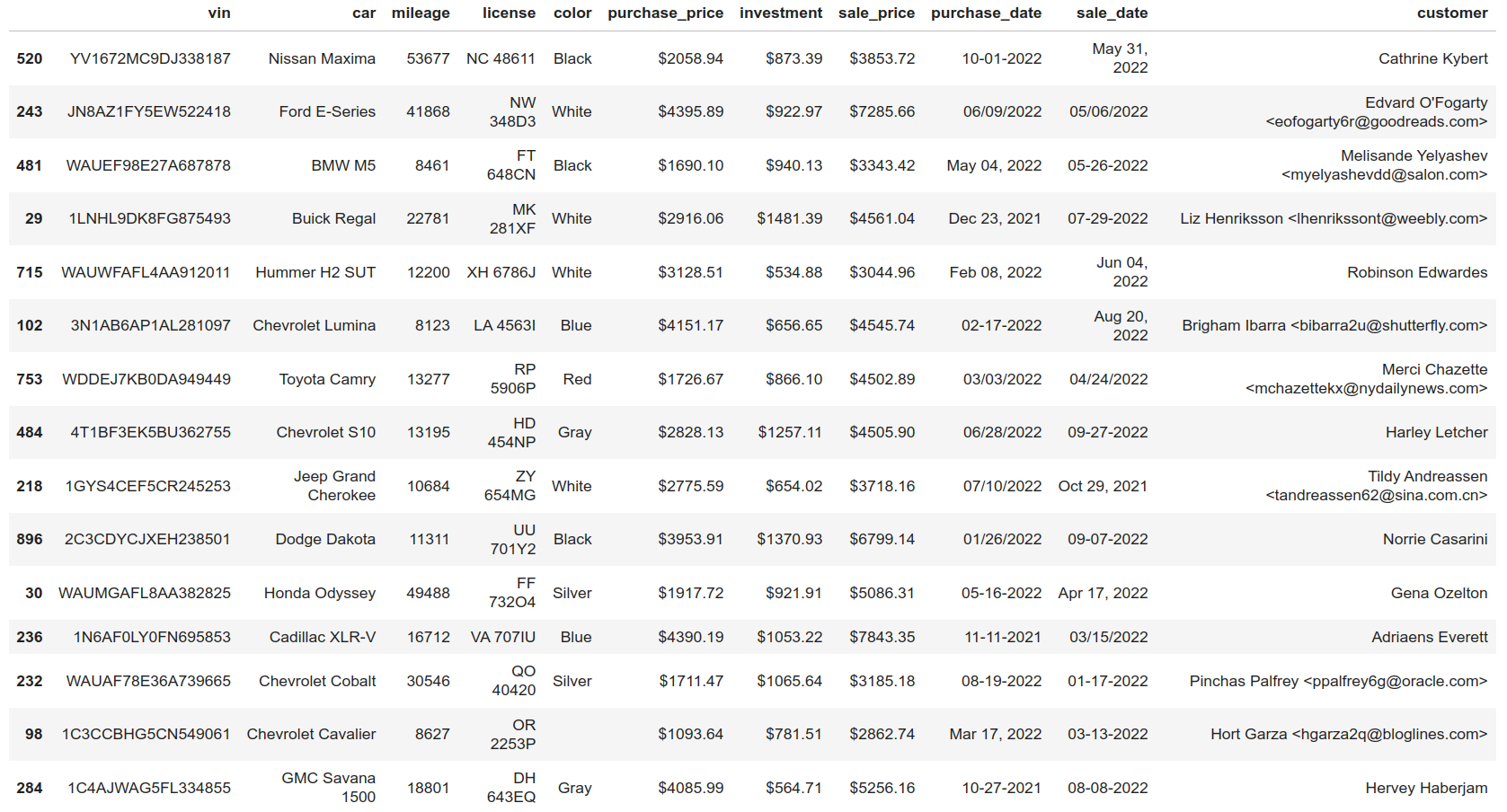
Before jumping into the code, it would help to explore your dataset to get a feel for what you’ll be dealing with. It’s going to be a single table consisting of used car dealership data stored in the car_sales.db file. Remember that you can download this sample dataset by clicking the link below:
Source Code: Click here to get the free source code and dataset that you’ll use to combine Python and Power BI for superpowered business insights.
There are a thousand records and eleven columns in the table, which represent sold cars, their buyers, and the corresponding sales details. You can quickly visualize this sample database by loading it into a pandas DataFrame and sampling a few records in a Jupyter Notebook using the following code snippet:
import sqlite3
import pandas as pd

with sqlite3.connect(r"C:\Users\User\Desktop\car_sales.db") as connection:
    df = pd.read_sql_query("SELECT * FROM sales", connection)

df.sample(15)
Note that the path to the car_sales.db file may be different on your computer. If you can’t use Jupyter Notebook, then try installing a tool like SQLite Browser and loading the file into it. Either way, the sample data should be represented as a table similar to the one below:
At a glance, you can tell that the table needs some cleaning because of several problems with the underlying data. However, you’ll deal with most of them later, in the Power Query editor, during the data transformation phase. Right now, focus on loading the data into Power BI.
As long as you haven’t dismissed the welcome screen in Power BI yet, then you’ll be able to click the link labeled Get data with a cylinder icon on the left. Alternatively, you can click Get data from another source on the main view of your report, as none of the few shortcut icons include Python. Finally, if that doesn’t help, then use the menu at the top by selecting Home › Get data › More… as depicted below:
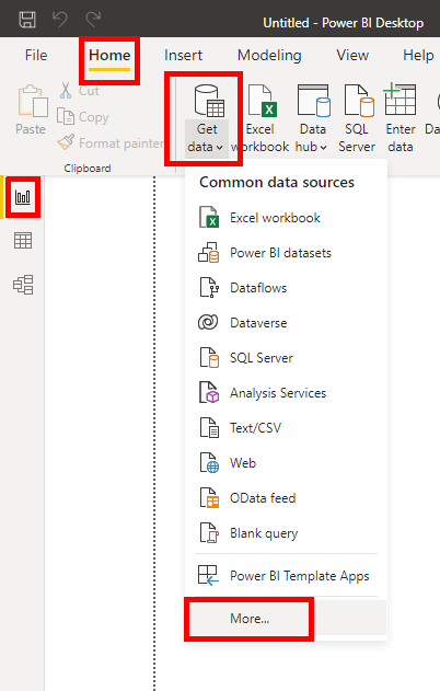
Doing so will reveal a pop-up window with a selection of Power BI connectors for several data sources, including a Python script, which you can find by typing python into the search box:
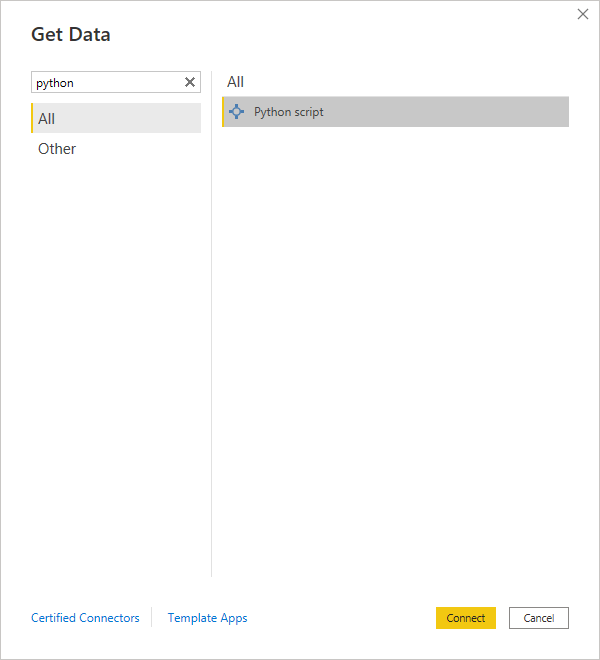
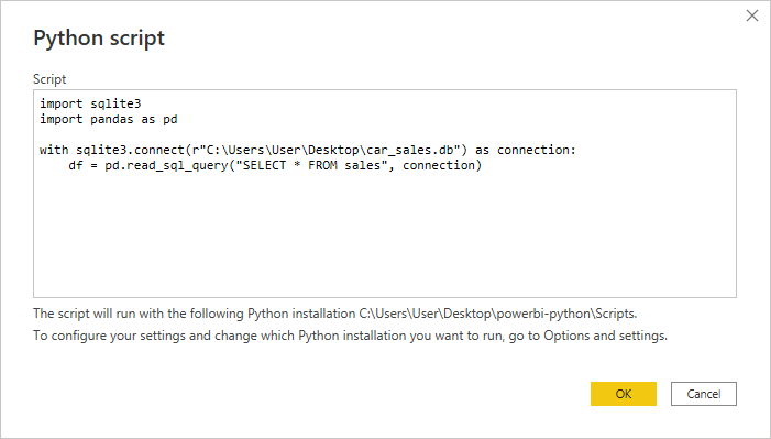
Select it and click the Connect button at the bottom to confirm. Afterward, you’ll see a blank editor window for your Python script, where you can type a brief code snippet to load records into a pandas DataFrame:
Notice the lack of syntax highlighting or intelligent code suggestions in the editor built into Power BI. As you learned earlier, it’s much better to use an external code editor, such as VS Code, to test that everything works as expected and only then paste your Python code to Power BI.
Before moving forward, you can double-check if Power BI uses the right virtual environment, with pandas and Matplotlib installed, by reading the text just below the editor.
While there’s only one table in the attached SQLite database, it’s currently kept in a denormalized form, making the associated data redundant and susceptible to all kinds of anomalies. Extracting separate entities, such as cars, sales, and customers, into individual DataFrames would be a good first step in the right direction to rectify the situation.
Fortunately, your Python script may produce as many DataFrames as you like, and Power BI will let you choose which ones to include in the final report. For example, you can extract those three entities with pandas using column subsetting in the following way:
import sqlite3
import pandas as pd

with sqlite3.connect(r"C:\Users\User\Desktop\car_sales.db") as connection:
    df = pd.read_sql_query("SELECT * FROM sales", connection)

cars = df[
    [
        "vin",
        "car",
        "mileage",
        "license",
        "color",
        "purchase_date",
        "purchase_price",
        "investment",
    ]
]
customers = df[["vin", "customer"]]
sales = df[["vin", "sale_price", "sale_date"]]
First, you connect to the SQLite database by specifying a suitable path for the car_sales.db file, which may look different on your computer. Next, you run a SQL query that selects all the rows in the sales table and puts them into a new pandas DataFrame called df. Finally, you create three additional DataFrames by cherry-picking specific columns. The vehicle identification number (VIN) works as a primary key by tying related records.
Note: It’s customary to abbreviate pandas as pd in Python code. Often, you’ll also see the variable name df used for general, short-lived DataFrames. However, as a general rule, please choose meaningful and descriptive names for your variables to make the code more readable.
When you click OK and wait for a few seconds, Power BI will present you with a visual representation of the four DataFrames produced by your Python script. Assuming there were no syntax errors and you specified the correct file path to the database, you should see the following window:
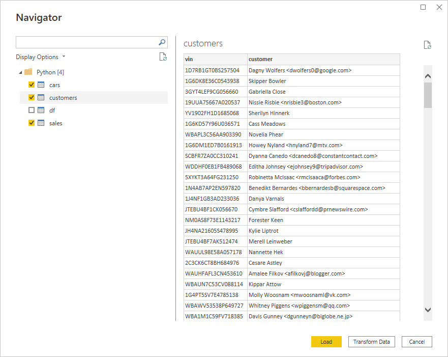
The resulting table names correspond to your Python variables. When you click on one, you’ll see a quick preview of the contained data. The screenshot above shows the customers table, which comprises only two columns.
Select cars, customers, and sales in the hierarchical tree on the left while leaving off df, as you won’t need that one. You could finish the data import now by loading the selected DataFrames into your report. However, you’ll want to click a button labeled Transform Data to perform data cleaning using pandas in Power BI.
Note: For more details on the topics in this section, check out Microsoft’s documentation on how to run Python scripts in Power BI Desktop.
In the next section, you’ll learn how to use Python to clean, transform, and augment the data that you’ve been working with in Power BI.
Power Query Editor: Transform and Augment Data
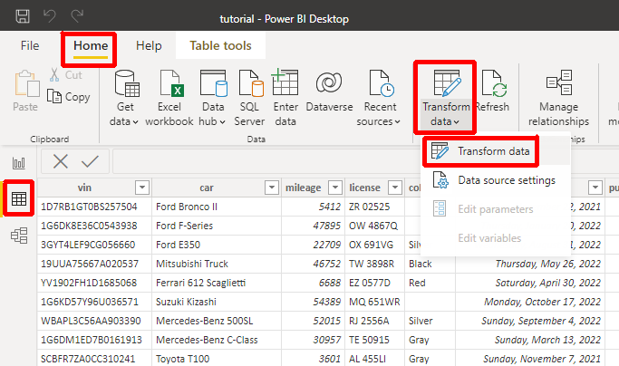
If you’ve followed the steps in this tutorial, then you should’ve ended up in the Power Query Editor, which shows the three DataFrames that you selected before. They’re called queries in this view. But if you’ve already loaded data into your Power BI report without applying any transformations, then don’t worry! You can bring up the same editor anytime.
Navigate to the Data perspective by clicking the table icon in the middle of the ribbon on the left and then choose Transform data from the Home menu:
Alternatively, you can right-click one of the Fields in the Data view on the far right of the window and choose Edit query for the same effect. Once the Power Query Editor window appears again, it’ll contain your DataFrames or Queries on the left and the Applied Steps on the right for the currently selected DataFrame, with rows and columns in the middle:
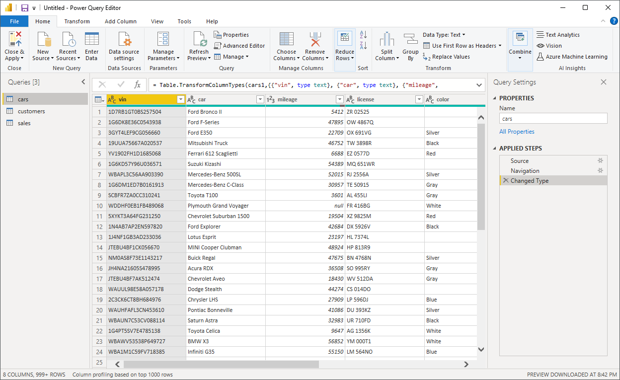
Steps represent a sequence of data transformations applied top to bottom in a pipeline-like fashion against a query. Each step is expressed as a Power Query M formula. The first step, named Source, was the invocation of your Python script that produced four DataFrames based on the SQLite database. The other two steps fish out the relevant DataFrame and then transform the column types.
Note: By clicking the gear icon next to the Source step, you’ll reveal the original Python source code of your data ingestion script. You can use this feature to access and edit Python code baked into a Power BI report even after saving it as a .pbix file.
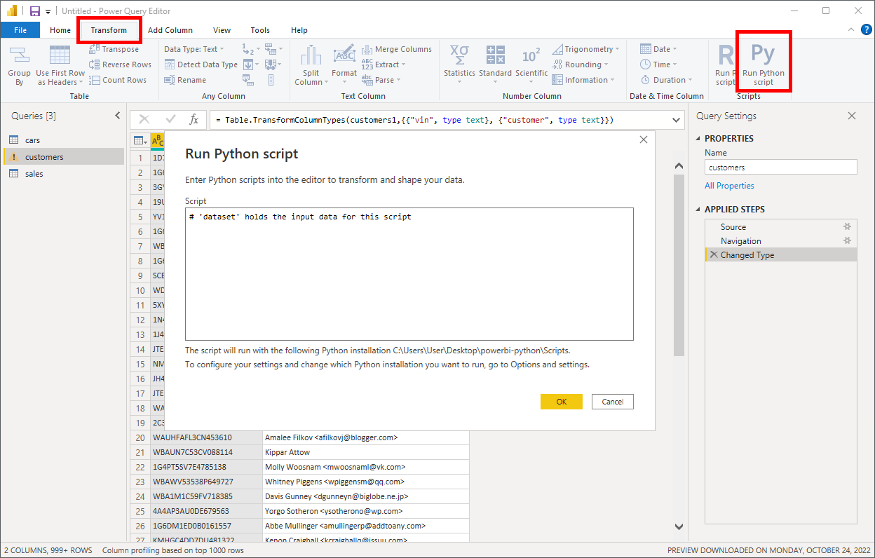
You can insert custom steps into the pipeline for more granular control over data transformations. Power BI Desktop offers plenty of built-in transformations that you’ll find in the top menu of Power Query Editor. But in this tutorial, you’ll explore the Run Python script transformation, which is the second mode of running Python code in Power BI:
Conceptually, it works almost identically to data ingestion, but there are a few differences. First of all, you may use this transformation with any data source that Power BI supports natively, so it could be the only use of Python in your report. Secondly, you get an implicit global variable called dataset in your script, which holds the current state of the data in the pipeline, represented as a pandas DataFrame.
Note: As before, your script can produce multiple DataFrames, but you’ll only be able to select one for further processing in the transformation pipeline. You can also decide to modify your dataset in place without creating any new DataFrames.
Pandas lets you extract values from an existing column into new columns using regular expressions. For example, some customers in your table have an email address enclosed in angle brackets (<>) next to their name, which should really belong to a separate column.
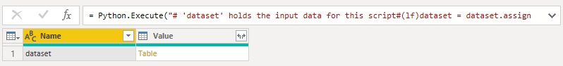
Select the customers query, then select the last Changed Type step, and add a Run Python script transformation to the applied steps. When the pop-up window appears, type the following code fragment into it:
# 'dataset' holds the input data for this script
dataset = dataset.assign(
    full_name=dataset["customer"].str.extract(r"([^<]+)"),
    email=dataset["customer"].str.extract(r"<([^>]+)>")
).drop(columns=["customer"])
Power BI injects the implicit dataset variable into your script to reference the customers DataFrame, so you access its methods and override it with your transformed data. Alternatively, you could define a new variable for the resulting DataFrame. During the transformation, you assign two new columns, full_name and email, and then remove the original customer column that contained both pieces of information.
After clicking OK and waiting for a few seconds, you’ll see a table with the DataFrames your script produced:
There’s only one DataFrame, called dataset, because you reused the implicit global variable provided by Power BI for your new DataFrame. Go ahead and click the yellow Table link in the Value column to choose your DataFrame. This will generate a new output of your applied steps:
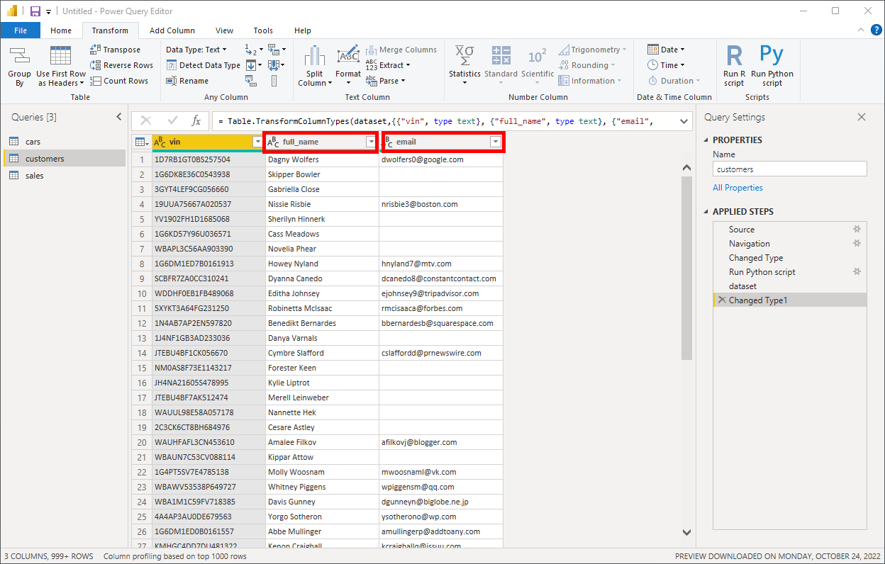
Suddenly, there are two new columns in your customers table. Now you can instantly find customers who haven’t provided their email addresses. If you want to, you can add more transformation steps to, for example, split the full_name column into first_name and last_name, assuming there are no edge cases with more than two names.
Make sure that the last step is selected, and insert yet another Run Python script into the applied steps. The corresponding Python code should look as follows:
# 'dataset' holds the input data for this script
dataset[
    ["first_name", "last_name"]
] = dataset["full_name"].str.split(n=1, expand=True)
dataset.drop(columns=["full_name"], inplace=True)
Unlike in the previous step, the dataset variable refers to a DataFrame with three columns, vin, full_name, and email, because you’re further down the pipeline. Also, notice the inplace=True parameter, which drops the full_name column from the existing DataFrame rather than returning a new object.
You’ll notice that Power BI gives generic names to the applied steps and appends consecutive numbers to them in case of many instances of the same step. Fortunately, you can give the steps more descriptive names by right-clicking on a step and choosing Rename from the context menu:
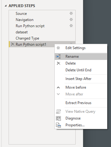
By editing Properties…, you may also describe in a few sentences what the given step is trying to accomplish.
There’s so much more you can do with pandas and Python in Power BI to transform your datasets! For example, you could:
- Anonymize sensitive personal information, such as credit card numbers
- Identify and extract new entities from your datasets
- Reject car sales with missing transaction details
- Remove duplicate sales records
- Synthesize the model year of a car based on its VIN
- Unify inconsistent purchase and sale date formats
These are just a few ideas. While there’s not enough room in this tutorial to cover everything, you’re more than welcome to experiment on your own and check out the bonus materials. Note that your success with using Python to transform data in Power BI will depend on your knowledge of pandas, which Power BI uses under the hood. To brush up on your skills, check out the pandas for Data Science learning path here at Real Python.
When you’re finished transforming your datasets, you can close the Power Query Editor by choosing Close & Apply from the Home ribbon or its alias in the File menu:
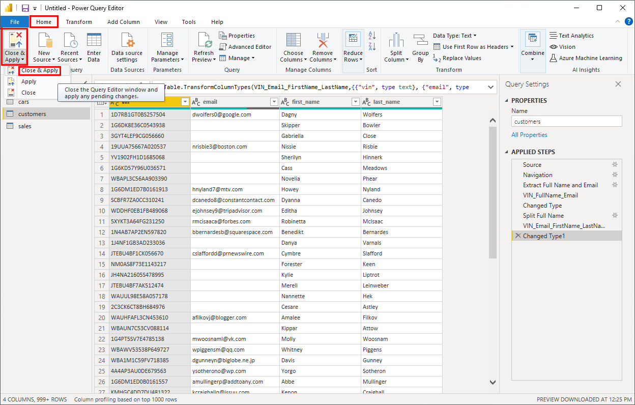
This will apply all transformation steps across your datasets and return to the main window of Power BI Desktop.
Note: For more details on the topics in this section, check out Microsoft’s documentation on how to use Python in Power Query Editor.
Next up, you’ll learn how to use Python to produce custom data visualizations.
Visuals: Plot a Static Image of the Data
So far, you’ve imported and transformed data. The third and final application of Python in Power BI Desktop is plotting the visual representation of your data. When creating visualizations, you can use any of the supported Python libraries as long as you’ve installed them in the virtual environment that Power BI uses. However, Matplotlib is the foundation for plotting, which those libraries delegate to anyway.
Unless Power BI has already taken you to the Report perspective after transforming your datasets, navigate there now by clicking the chart icon on the left ribbon. You should see a blank report canvas where you’ll be placing your graphs and other interactive components, jointly named visuals:
Over on the right in the Visualizations palette, you’ll see a number of icons corresponding to the available visuals. Find the icon of the Python visual and click it to add the visual to the report canvas. The first time you add a Python or R visual to a Power BI report, it’ll ask you to enable script visuals:
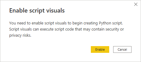
In fact, it’ll keep asking you the same question in each Power BI session because there’s no global setting for this. When you open a file with your saved report that uses script visuals, you’ll have the option to review the embedded Python code before enabling it. Why? The short answer is that Power BI cares for your privacy, as any script could leak or damage your data if it’s from an untrusted source.
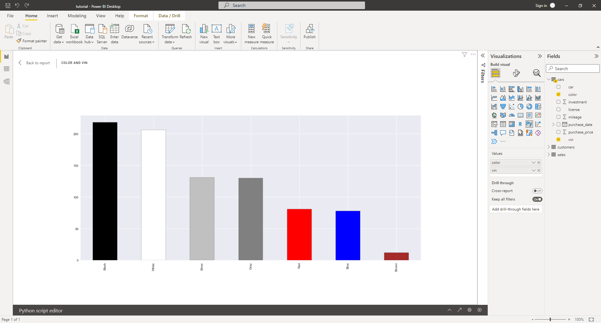
Expand your cars table in the Fields toolbar on the right and drag-and-drop its color and vin columns onto the Values of your visual:
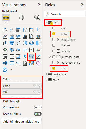
These will become the only columns of the implicit dataset DataFrame provided by Power BI in your Python script. Adding those data fields to a visual’s values enables the Python script editor at the bottom of the window. Somewhat surprisingly, this one does offer basic syntax highlighting:
However, if you’ve configured Power BI to use an external code editor, then clicking on the little skewed arrow icon (↗) will launch it and open the entire scaffolding of the script. You can ignore its content for the moment, as you’ll explore it in an upcoming section. Unfortunately, you have to manually copy and paste the script’s part between the auto-generated # Prolog and # Epilog comments back to Power BI when you’re done editing.
Note: Don’t ignore the yellow warning bar in the Python script editor, which reminds you that rows with duplicate values will be removed. If you only dragged the color column, then you’d end up with just a handful of records corresponding to the few unique colors. However, adding the vin column prevents this by letting colors repeat throughout the table, which can be useful when performing aggregations.
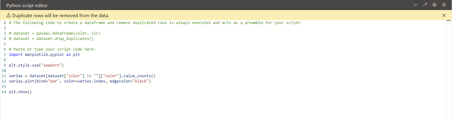
To demonstrate an elementary use of a Python visual in Power BI, you can plot a bar chart showing the number of cars painted a given color:
# The following code to create a dataframe and remove duplicated
# rows is always executed and acts as a preamble for your script:

# dataset = pandas.DataFrame(color, vin)
# dataset = dataset.drop_duplicates()

# Paste or type your script code here:
import matplotlib.pyplot as plt

plt.style.use("seaborn")

series = dataset[dataset["color"] != ""]["color"].value_counts()
series.plot(kind="bar", color=series.index, edgecolor="black")

plt.show()
You start by enabling Matplotlib’s theme that mimics the seaborn library for a slightly more appealing look and feel compared to the default one. Next, you eliminate records with a missing color and count the remaining ones in each unique color group. This produces a pandas.Series object, which you can plot and color-code using its index consisting of the color names. Finally, you call plt.show() to render the plot.
To trigger this code for the first time, you must click the play icon in the Python script editor, as you haven’t displayed any data in your report. If you’re getting an error about no images having been created, then check if you called plt.show() at the end of your script. It’s necessary so that Matplotlib renders the plot on the default backend, which means writing the rendered PNG image to a file on disk, which Power BI can load and display.
As long as everything goes fine, your blank report should gain some colors:
You can move and resize the visual to make it bigger or change its proportions. Alternatively, you may enter Focus mode by clicking a relevant icon on the visual, which will expand it to accommodate the available space.
Python visuals automatically update in response to changes in data, filtering, and highlighting, just like other Power BI visuals. However, the rendered image itself is static, so you can’t interact with it in any way to cross-filter other visuals. To test how filtering works, go ahead and add a Slicer next to your visual with the car’s purchase_date data field:
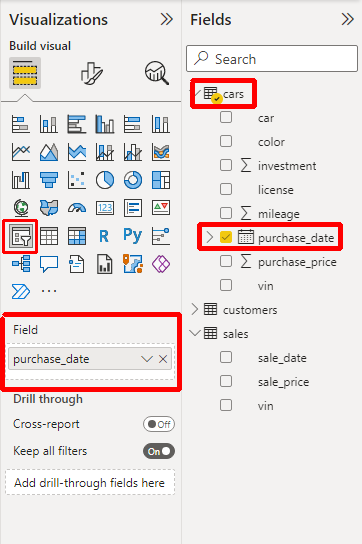
It’ll create an interactive slider widget in your report that’ll let you tweak the range of dates of car purchases. Every time you adjust those dates, Power BI will rerun your Python script to produce a new static rendering of the data, which admittedly takes a few moments to update:
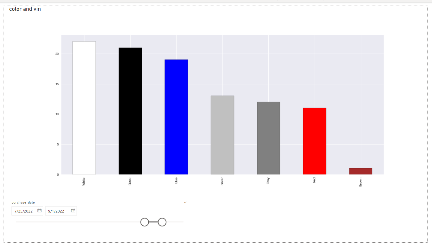
Notice that the color distribution on the visual has changed slightly. Apart from slicing the data, you could also define a filter in Power BI to, for example, only show car colors for a particular brand, as determined by a VIN prefix.
Note: For more details on the topics in this section, check out Microsoft’s documentation on how to create Power BI visuals by using Python.
Python visuals in Power BI are merely static images with a resolution limited to 72 DPI. They aren’t interactive, and they take some time to update. Nevertheless, despite those limitations, they can enrich your palette of existing visuals in Power BI.
Now that you have hands-on experience using Python in Power BI Desktop, it’s time to dive deeper. In the next section, you’ll understand how the integration of both tools works by peeking under the surface.
Understanding the Integration of Power BI and Python
Knowing how to handle a tool can give you valuable skills. However, knowledge of the tool’s internals is what gives you true power to become proficient. Read on to learn how exactly Power BI Desktop integrates with Python and other scripting languages.
Intercept Power BI’s Temporary Files
Power BI controls the whole process of working with your report’s data, so it’s in charge of running Python code and interfacing with it in both directions. In particular, Power BI needs to supply the script with a DataFrame to transform or visualize, and it needs to load DataFrames or visualizations from that script.
What’s one of the most straightforward mechanisms to facilitate such an interface between foreign programs?
If you think about it for a moment, then you may realize that you use that mechanism all the time. For example, when you make a spreadsheet in Microsoft Excel or other software, you save it in an .xlsx file that other programs can read, provided that they understand that particular data format. It may not be the most efficient way of sharing data across applications, but it’s pretty reliable.
Power BI uses a similar approach of leveraging the file system to communicate with your Python scripts. However, it does so in an automated and slightly more structured way. Each time Power BI wants to execute a Python script, it creates a temporary folder with a unique pseudo-random name in your user folder, as so:
C:\Users\User\PythonScriptWrapper_a6a7009b-1938-471b-b9e4-a1668a38458a
│
├── cars.csv
├── customers.csv
├── df.csv
├── sales.csv
├── input_df_738f5a98-23e4-4873-b00e-0c5780220bb9.csv
└── PythonScriptWrapper.PY
The folder contains a wrapper script with your Python code inside. It may also include a CSV file with the input dataset, which the script will load into the dataset variable if the associated step isn’t the first one in the pipeline. After executing, the wrapper script automatically dumps your DataFrames to CSV files named after the corresponding global variables. These are the tables that Power BI will let you choose for further processing.
The folder and its contents are only temporary, meaning they disappear without leaving any traces when they’re no longer needed. Power BI removes them when the script finishes executing.
The wrapper script contains the glue code that takes care of data serialization and deserialization between Power BI and Python. Here’s an example:
# Prolog - Auto Generated #
import os, pandas, matplotlib
matplotlib.use('Agg')
import matplotlib.pyplot

import sys
sys.tracebacklimit = 0

os.chdir(u'C:/Users/User/PythonScriptWrapper_a6a7009b-1938-471b-b9e4-a1668a38458a')
dataset = pandas.read_csv('input_df_738f5a98-23e4-4873-b00e-0c5780220bb9.csv')

matplotlib.pyplot.show = lambda args=None,kw=None: ()
POWERBI_GET_USED_VARIABLES = dir
# Original Script. Please update your script content here and once completed copy below section back to the original editing window 'dataset' holds the input data for this script

# ...

# Epilog - Auto Generated #
os.chdir(u'C:/Users/User/PythonScriptWrapper_a6a7009b-1938-471b-b9e4-a1668a38458a')
for key in POWERBI_GET_USED_VARIABLES():
 if (type(globals()[key]) is pandas.DataFrame):
  (globals()[key]).to_csv(key + '.csv', index = False)
The highlighted line is optional and will only appear in the intermediate or terminal steps of the pipeline, which transform some existing datasets. On the other hand, a data ingestion script, which corresponds to the first step, won’t contain any input DataFrames to deserialize, so Power BI won’t generate this implicit variable.
The wrapper script consists of three parts separated with Python comments:
- Prolog: Deserialization of the input CSV to a DataFrame, and other plumbing
- Body: Your original code from the Python script editor in Power BI Desktop
- Epilog: Serialization of one or more DataFrames to CSV files
As you can see, there’s a substantial input/output overhead when using Python in Power BI because of the extra data marshaling cost. To transform a single piece of data, it has to be serialized and deserialized four times, in this order:
- Power BI to CSV
- CSV to Python
- Python to CSV
- CSV to Power BI
Reading and writing files are expensive operations and can’t compare to directly accessing a shared memory in the same program. Therefore, if you have large datasets and performance is vital to you, then you should prefer Power BI’s built-in transformations and the Data Analysis Expression (DAX) formula language over Python. At the same time, using Python may be your only option if you have some existing code that you’d like to reuse in Power BI.
The wrapper script for plotting Power BI visuals with Python looks very similar:
# Prolog - Auto Generated #
import os, uuid, matplotlib
matplotlib.use('Agg')
import matplotlib.pyplot
import pandas

import sys
sys.tracebacklimit = 0

os.chdir(u'C:/Users/User/PythonScriptWrapper_0fe352b7-79cf-477a-9e9d-80203fde2a54')
dataset = pandas.read_csv('input_df_84e90f47-2386-45a9-90d4-77efca6d4942.csv')

matplotlib.pyplot.figure(figsize=(4.03029540114132,3.76640651225243), dpi=72)
matplotlib.pyplot.show = lambda args=None,kw=None: matplotlib.pyplot.savefig(str(uuid.uuid1()))
# Original Script. Please update your script content here and once completed copy below section back to the original editing window #
# The following code to create a dataframe and remove duplicated rows is always executed and acts as a preamble for your script:

# dataset = pandas.DataFrame(car)
# dataset = dataset.drop_duplicates()

# Paste or type your script code here:

# ...

# Epilog - Auto Generated #
os.chdir(u'C:/Users/User/PythonScriptWrapper_0fe352b7-79cf-477a-9e9d-80203fde2a54')
The generated code overwrites Matplotlib’s plt.show() method so that plotting the data saves the rendered figure as a PNG image with a resolution of 72 DPI. The width and height of the image will depend on the dimensions of your visual in Power BI. The input DataFrame may contain a filtered or sliced subset of the complete dataset.
That’s how Power BI Desktop integrates with Python scripts. Next, you’ll learn where Power BI stores your Python code and data in a report.
Find and Edit Python Scripts in a Power BI Report
When you save a Power BI report as a .pbix file, all the related Python scripts get retained in a compressed binary form inside your report. You can edit those scripts afterward to update some datasets or visuals if you want to. However, finding the associated Python code in Power BI Desktop can be tricky.
To reveal the source code of a Python visual, click on the visual itself when viewing it on the report canvas. This will display the familiar Python script editor at the bottom of the window, letting you make changes to the code instantly. Power BI will run this new code when you either interact with other visuals and filters or when you click the play icon in the Python script editor.
Finding the Python code of your data ingestion or transformation scripts is a bit more challenging. First, you must bring up Power Query Editor by choosing Transform data from the menu on the Data perspective, just like you did when you performed data transformation. Once there, locate an applied step that corresponds to running a piece of Python code. It’s usually named Source or Run Python script unless you renamed that step.
Then, click on the gear icon next to the appropriate step or choose the Edit Settings option from its context menu to show your original Python code. After editing and confirming the updated code by clicking OK, you’ll have to indicate which resulting table to choose for further processing. When you do, you may see the following warning appear in Power BI:
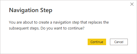
You’ll see this warning when there are subsequent steps below the one you’ve just edited. In such a case, your change could affect the rest of the applied steps pipeline. So, if you click Continue now, then Power BI will remove the following steps. However, if you change your mind and want to discard pending changes, then you’ll still be able to close the Power Query Editor window without applying them.
When you do introduce a change to one of your Python scripts in Power Query Editor and apply it, then Power BI will try to refresh the corresponding dataset by pushing it through the entire pipeline again. In other words, you have to be able to access your original data source, such as the SQLite database, or else you’ll get an error.
Note: Apart from the scripts, Power BI keeps your ingested and transformed datasets in the .pbix file. So, unless you edit a data-related Python script, you can start interacting with your report right away after opening it.
At this point, you know what is achievable with Python in Power BI and how the integration between them works on a lower level. In the final section of this tutorial, you’ll take a closer look at some of the limitations stemming from this integration, which may help you make an informed decision about when to use Python in Power BI.
Considering the Limitations of Python in Power BI
In this section, you’ll learn about the limitations of using Python in Power BI Desktop. The most strict limitations concern Power BI visuals rather than the data-related scripts, though.
Timeouts and Data Size Limitations
According to the official documentation, your data ingestion and transformation scripts defined in Power Query Editor can’t run longer than thirty minutes, or else they’ll time out with an error. The scripts in Python visuals are limited to only five minutes of execution, though. If you’re processing really big datasets, then that could be a problem.
Furthermore, Python scripts in Power BI visuals are subject to additional data size limitations. The most important ones include the following:
- Only the top 150,000 rows or fewer in a dataset can be plotted.
- The input dataset can’t be larger than 250 megabytes.
- Strings longer than 32,766 characters will be truncated.
Time and memory are limited in Power BI when running Python scripts. However, the actual Python code execution also incurs a cost, which you’ll learn about now.
Data Marshaling Overhead
As you learned earlier, Power BI Desktop communicates with Python by means of exchanging CSV files. So, instead of manipulating the dataset directly, your Python script must load it from a text file, which Power BI creates for each run. Later, the script saves the result to yet another text or image file for Power BI to read.
This redundant data marshaling results in a significant performance bottleneck when working with larger datasets. It’s perhaps the biggest drawback of Python integration in Power BI Desktop. If the poor performance becomes noticeable, then you should consider using Power BI’s built-in transformations or the Data Analysis Expression (DAX) formula language over Python.
Alternatively, you may try reducing the number of data serializations by collapsing multiple steps into one Python script that does the heavy lifting in bulk. So if the example you worked through at the beginning of the tutorial was for a very large dataset, instead of making multiple steps in the Power Query Editor, you would be best off trying to combine them into the first loading script.
Non-Interactive Python Visuals
Data visualizations that use Python code for rendering are static images, which you can’t interact with to filter your dataset. However, Power BI will trigger the update of Python visuals in response to interacting with other visuals. Additionally, Python visuals take slightly longer to display because of the previously mentioned data marshaling overhead and the need to run Python code to render them.
Other Minor Nuisances
There are also a few other, less significant limitations of using Python in Power BI. For example, you can’t easily share your Power BI reports with others if it would require them to install and configure Python. The privacy levels of all the datasets in a report must be set to public for Python scripts to work correctly in the Power BI service. There’s a finite number of supported Python libraries in Power BI. The list goes on.
For a more complete overview of the limitations of Python in Power BI, check out how to prepare a Python script and the known limitations of Python visuals in Microsoft’s documentation.
Conclusion
Even if you haven’t used Python or Power BI before, you can now combine both tools in your data analysis workflow. You successfully loaded data into your Power BI report from a SQLite database using Python, and you took advantage of the pandas library to transform and augment your dataset. Finally, you visualized the data in Power BI by plotting it with Python’s Matplotlib.
In this tutorial, you learned how to:
- Install and configure the Python and Power BI environment
- Use Python to import and transform data
- Make custom visualizations using Python
- Reuse your existing Python source code
- Understand the limitations of using Python in Power BI
You’re now equipped with the knowledge to leverage two powerful technologies, Power BI and Python, to transform how you make data-driven business decisions!
Source Code: Click here to get the free source code and dataset that you’ll use to combine Python and Power BI for superpowered business insights.